Retail Shrink

Retail Shrink is defined as the difference between the value of goods available as per the books and the actual value of goods available in the retail store. For example, a retailer might be thinking that there are 50 bottles of 500 ml Pepsi soft drink as per the records. But in reality, there might only be 48 bottles. The cost of the two missing bottles is the shrinkage value.

Retail shrink is not just about physical reduction in quantity of an SKU. Let me cite another example. A store employee can manipulate the POS by adjusting the discount % given to certain goods, thus registering an incorrect sale value in the system. Another example could be registering a fraudulent return of a product, thus incrementing the number of SKUs in the store and taking away the equivalent cash. In simple language any fraudulent activity that results in monetary loss to the retailer contributes to retail shrinkage.

A survey states that in 2011, the global retail shrinkage stands at more than $100 Billion. The sheer magnitude of the money involved explains the importance that retail shrinkage has in modern retail. There are a variety of reasons for why shrinkage happens. Some of the common causes are:

1)      Shoplifting

2)      Employee theft

3)      Vendor fraud

4)      Administrative Errors

Shoplifting is a common known factor and is being arrested by the retailers by deploying scanners in the store exits

Employee theft is a difficult factor to address. The stores can be successful in restricting the employees taking away products from the backroom of the store or the warehouse by imposing stricter physical security measures, but when employees indulge in manipulation of POS, it becomes little tricky to handle.

Vendor fraud occurs most when 3^rd party vendors are allowed to stock / unstock their products inside the store.

Administrative errors occur when by mistake, an incorrect value is being entered into the store inventory management system. Such issues can be minimized by the use of electronic scanners / PDAs for entering the stock quantities into the inventory management systems.

Hope this gives a brief and clear overview of what retail shrinkage is and how it is caused.

 

Order to cash

“Order to Cash” refers to the set of business processes that starts from the point when a customer places an order, to the state when the customer pays for the goods received. A typical Order to Cash (commonly termed OTC) cycle looks like the following:

Place an Order: This is the phase when the customer places an order with the supplier or vendor. An example of this could be:

1)      A retailer placing an order for 10 cartons of washing powder, each containing 20 packets of 500 grams each

There are multiple ways in which such orders are placed. The vendor and the customer can have access to a common internet portal. There are channels like EDI (Electronic Data Interchange), which provide a standard way to transmit data between organizations.

Reconcile an order: Once an order is placed, the duty of the vendor is to validate the order for completeness. There is also a need to check the credit worthiness of the customer, who places the order. The checks could be such as

1)      Whether the customer has paid all the past dues or not,

2)      Whether the dollar amount involved in the transaction is abnormal or not etc.

Fulfill an order: This is the process that takes care of fulfilling the order placed by the customer. Fulfilling is about planning and executing an efficient order delivery process. The end result of this process is to transmit the goods to consumers based on the order request, but there is lot of planning involved in terms of sequencing the order transmission and consolidating the orders placed by multiple customers. For example,

1)      There could be restrictions around sending a specific product. A customer might have placed an order for 50 cartons of a specific product. But the vendor might be able to send only 25 cartons at any given time.

2)      There could be orders for a specific product from multiple customers but in small quantities. This gives a scope to consolidate the orders and send as one master shipment till some location and then dividing the goods for last mile delivery

Invoicing: This is the process which handles the generation and delivery of invoices to the customers. These invoices are generally electronically generated and sent through channels like EDI (just as how orders are placed). Otherwise they could be transmitted even by means of internet portals accessible by vendors and customers. These invoices are generally used by the customers to match against the orders they placed and the goods that they received

Payments processing: Once the goods are received, the customers will execute a reconciliation process to match the orders they placed against the goods received and the invoices. If the reconciliation proves good, the customer will release the payment to the vendors. This financial transaction is recorded in the accounting systems (such as General Ledger) of both vendor and the customer. There will be credit policies agreed upon between both these parties which govern the payments. For example, there could be an agreement that states payment will be made within 30 days after the goods are received by the customer. When such terms and conditions regarding the payment are violated, then the “Collections” department may come into the picture to facilitate the collection of payments from customers.

Hope this gives a simplistic overview of the Order-To-Cash cycle. These processes are handled in a sophisticated manner by various Enterprise Resource Planning (ERP) packages such as SAP. These ERP packages have been successful over the years in articulating the needs to customers from various industries and satisfying their requirements by and large.

Feel free to register your comments, if you have any feedback.

 

Long-tail effect

Many research papers and articles have been written by experts on possible existence and illusion of long tail effect in the retail industry, specific to e-commerce. This post is a primitive attempt to simplify the long tail effect such that it can be easily comprehended by a beginner in retail industry.

Traditionally, the belief is that 20% of the products stocked by a retailer contributes to 80% of the sales revenue. i.e. More popular goods are sold very frequently (compared to uncommon or unpopular ones) and they generate most of a retailer’s revenue. By and large, this had been true on many cases, but the evolution of e-commerce in retail has shaken this belief to a reasonable extent. In-Store retailers always had the limitation of stocking only fast moving goods in stores to ensure that they don’t waste the shelf-space. However, this limitation is no longer true for many e-commerce firms, especially for the ones such as Netflix & Amazon (The oft-quoted examples).

Let us take the example of Netflix. If there is a physical store that rents out movies, then it can probably store a few thousand DVDs in the store depending on the store capacity. And it can stock only those movies which are quite popular and that can be easily rented out. However, an e-commerce company like Netflix can store at least 10 times more DVDs than such a physical store, in a centralized warehouse and if there is even a smaller demand for the unpopular DVDs, the revenue that it can generate by renting out such movies is very high.

In the Indian context, there are a few examples as well. Let us take an e-commerce firm such as Myntra.com, which is an online fashion retailer. The catalogue of dresses or shoes (for instance) in that website is pretty huge compared to a physical store, which gives the consumer an option to search more and choose the one that he/she likes the most. The cost of searching is less and the storage costs are not way too high, which enable a firm like Myntra to get benefitted by selling unpopular goods, which are not found in every other store.

However, there are 2 factors that primarily decide whether an e-commerce firm can really get benefited by this long-tail effect.

1. Costs involved in maintaining the supply chain – This concept will hold good only if the storage and distribution costs for the long tail of products is not expensive. I.e. This will be beneficial in case of e-commerce rental services which stock movie DVDs or firms that sell products such as books, dresses & apparels. Generally, long tail effect is not going to help a retailer who’s into selling perishable products.

1. Consumer behavior – The trick lays in predicting the right consumer demand patterns. It should be noted that the tail of products should not only be long but also should be able to draw customer’s attention to trigger a purchase.

 

Store Site Selection

Site Selection for new stores

When a retailer starts off with the first store opening, there will not be much confusion about the potential location for the store site. The same situation may continue perhaps for the initial few stores. But when the number of stores owned by a retailer increases, or the number of franchisees increases, locating the right site for the new store (fully-owned or franchisee-owned) becomes a crucial decision for the top management of a retail firm. Reilly’s law of retail gravitation states that the attraction of a consumer to a given retailer is directly proportional to the quality of retailer and inversely proportional to the distance to the retailer. Though the basic premise is very true, in the current competitive landscape, there are many more factors (apart from the distance) that decide the attractiveness of a store. This post is intended to describe about the common factors that a retailer should consider while selecting a site for new store. As had been mentioned in the other posts, software products are readily available for this business problem as well. Especially there are many GIS (Geographical Information Systems) products in the market that help the management team to take decisions about this. But what works for one firm may not work for another. The reasons are quite obvious. Different retailers have different concepts and strategies. The reason for setting up a new store may be to increase revenues or to mitigate risk or to annihilate competition. The profit margins expected by different retailers may be different. The quantity of market share targeted by different firms will be different.

Let us try to understand more about Site Selection.

One of the elementary techniques in scientific site selection is to find sites that are more like existing sites. I.e. To determine locations that are similar to other existing store sites in terms of demographics and consumer purchase pattern. The demographic variables could be consumer age distribution, income levels and population density etc., A GIS tool loaded with adequate information can do such analysis by processing the demographic data for a particular radius around existing store sites. This can be compared with the results of similar analysis run against the proposed new store site.

Another scientific technique that is quite popular is to find the attributes that are linked to high sales revenue and look for sites that have those attributes. For example, we can find out the attributes that are highly positively correlated with increased sales. The attributes could be high education of surrounding population, adjacency to office locations, floor space of the store etc. Certain attributes such as the distance of the store from a market zone or adjacency to competitor’s store could be highly negatively correlated with increased sales. Proposed site locations can also be scored on these attributes and the final selection can be made based on those sites that scored well in all the attributes. The following figure shows a sample visual representation of the same. Here, a GIS tool highlights those locations which scored well in red and those that scored poor in blue. This also indicates the competitor’s site locations in circles.

In few other cases, the management preselects the area based on the fast growing nature or the locations which are developing fast in terms of economy or residential or commercial real estate etc. For doing such a pre-selection as well, GIS tools provide accurate data especially when there are many such locations which on the outset look similar.

As we can observe, the GIS tools used for such analysis are highly dependent on the data loaded onto them.

• Demographic data can be obtained from government statistical institutes, population census data etc. Agencies like Code-1 plus in US can also provide such information. Other syndicate agencies like Nielsen can provide information on customer buying pattern, sales trend etc.
• The company’s own database will have past sales information and the location of their existing stores. Information about the location of competitors’ stores and the location of business establishments such as schools, hospitals, movie theatres, parks, tourist attractions etc should also be loaded into the GIS tool.
• More importantly, the data about the customers’ origin should be known. Ie. Place from where customers come to the stores. Such data can be obtained from surveys, feedback forms, customer data from a retailer’s database etc.

All these are used by GIS products to do the required analysis and present the data in graphical formats that help the senior management to take decisions.

However, site selection becomes all the more complicated nowadays because of many reasons.

• For instance, when a company wants to set up a store in a market where the firm already has existing stores, not only should competition be considered, but cannibalization of existing store sales becomes a problem as well.
• Another reason for why site selection is complex is as follows. A certain number of residents located out of a market zone could be the customers of stores located in that market zone. Similarly, residents near a boundary of a market zone may be the customers of the stores in adjacent market zone.
• Also, many of the demographic data are highly dynamic. Age profile of customers, Average household size, average income level, consumers’ sophistication in terms of mobility – all change year after year.

Retailers should be well aware of these factors and make effective use of GIS products to take wise decisions about Store Site Selection. State of the art products are available now, which can provide such information as sales trend, customer demographic variations and the results of the analysis outlined above – all in 3-D format and in appealing GUI. Such tools have high potential to store and analyse volumes of information on various parameters in spatial (related to space/geography) and temporal (those that change with time) dimensions and propose suggestions about site selection. This information will be highly useful for managers to take appropriate decisions with respect to selecting the right location for the next store.

I hope that this post gave a basic understanding about how the problem of Site Selection is generally approached.

 

Multi-Echelon Inventory Management

Multi-Echelon Inventory System in a Real World

How to determine safety stock and reorder point at multiple levels in a multi-echelon inventory system?

To start with, let us assume that there is only one entity at each echelon and then we shall develop the concept if there are multiple entities in each echelon.

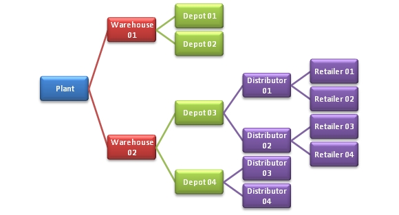
Here we should be aware that the echelon inventory at each level is equal to the inventory on hand at the echelon plus all downstream inventories. For example, the echelon inventory at the distributor level is equal to the inventory level at the distributor plus inventory level in transit to the retailer plus the inventory that is in stock at the retailer. When we say “echelon inventory position” at the distributor, then that would include the echelon inventory at the distributor plus the order that is yet to be received by the distributor minus the backorders for the distributor.

In this case, at the retailer level, inventory can be managed using a simple fixed order quantity. Ie., Whenever the echelon inventory position at the retailer falls to “R”, then a fixed quantity of “Q” can be ordered.

Where R is the reorder point and can be calculated using the following formula:

R = (LT * D_Avg)+ (Z *  Std * SQRT[LT])

Where,

LT = Lead Time between when the retailer places an order to the distributor and when the order is received

D_Avg  = Average Demand at the retailer

Z = Z-Value calculated based on the expected service level.

Std = Standard Deviation of the demand at the retailer

And Q = SQRT(2*D*S/H)

Where D = Annual Demand, S = Ordering Cost, H = Holding Cost per unit per year.

On a similar fashion, the Reorder point and the Order quantity for the upstream levels can also be calculated using the same formulae. But the only difference is in the way Lead Time is calculated for upstream levels. If we want to use the Reorder point formula for distributor, then the LT should be the lead time between the retailer and the distributor plus the lead time between the distributor and its supplier, which is depot in this case. Suppose the lead time is 1 week at all levels, then the lead time that should be used for calculating the reorder point at retailer level should be 1 week, whereas the lead time that should be used for calculating the reorder point at distributor level should be 2 weeks, the LT at Depot should be 3 weeks and so on. Other than this, the values of D_Avg and Std will remain the same at all levels.

Now let us see if there are multiple entities at each level – say one distributor catering to multiple retailers and one depot catering to multiple distributors.

Even in this case, the same procedure suggested above could be used, but with one subtle difference. The echelon inventory at each level would be the inventory in hand plus the inventory in transit to and in stock at all the entities at the next downstream level. For instance, the echelon inventory of Distributor 01 would be equal to the inventory in hand at Distributor 01 plus inventory in transit to Retailer 01 and Retailer 02 and inventory in stock at Retailer 01 and Retailer 02. Similarly, the echelon inventory position is equal to the sum of echelon inventory and the items that are ordered and not arrived, minus all the backorders.

To manage the inventory in such a system, whenever the echelon inventory position R is reached, an order should be placed for Q. For instance, the value of R the distributor can be calculated as,

R = (LT * D_Avg)+ (Z *  Std * SQRT[LT])

In this case,

D_Avg  = Average Demand across all the retailers (Average of aggregate demand)

Z = Z-Value calculated based on the expected service level.

Std = Standard Deviation of the aggregate demand across all the retailers.

LT = Echelon lead time, which is the lead time between retailers and the distributor plus the lead time between the distributor and depot.

This methodology can be extended to more complex supply chains as well, but the major challenge in implementing such a procedure is that the inventory information at all levels of the echelon should be known and the inventory control should be highly centralized.

 

Price Optimization

In this post, let me try to present some basics of pricing strategies and price optimization. One would agree that right pricing is of great significance to a retailer to succeed in today’s competitive landscape. This post would touch upon the broadly followed practices of pricing and the factors influencing pricing decisions of a retailer. I’ll try to document more about the role that analytics has to play in price optimization in another post.

Basics of Pricing

The very basic pricing method is to add a mark up to the cost involved in production, distribution & transportation of a particular SKU. For instance, the cost of raw materials, the variable cost per unit of production and SGA (Selling, General & Administrative Expenses) constitute the cost of an SKU. The retailer may wish to add a mark up of (say) 30% in addition to the cost incurred and fix the price.

The evolution of such a basic pricing mechanism led to rule based pricing techniques. For instance, a retailer may have a rule based engine that will decide upon the price of various categories of SKUs like the following example:

If the PRODUCT CATEGORY = ICE CREAMS,

1. Set MARKUP = 15%;
2. Set Last Digit of the Price = ‘9’;
3. Set Price = 95% of Competitor’s price; (5% less than competitor)
4. Set Private Label Ice Cream Brands = 80% of Popular brands; (20% less than popular ice cream brands)

In advanced systems that employ analytics to optimize the price of various SKUs, we can see even more sophistication, for example to do a “What If” Analysis, to determine the effect of a price change on the sales etc. Whatever be the tool deployed to optimize price, the retailer needs to be aware of certain key attributes that have a direct bearing on the way prices are fixed. Let us see that in the following section.

Factors influencing pricing decisions

As we know, a retailer has hundreds and thousands of SKUs in a store and there should be a way to manage the price of all these SKUs by some automated means. Though there is an MRP fixed by the manufacturer of the products, the retailer may wish to consider the following factors (not exhaustive) before fixing the price of that SKU in a particular store.

• Demand for the product
• Change in product mix and/or prices
• Regional influence on price
• Competitor’s pricing strategies
• Economic Conditions

Let us try and understand how these factors play a role in fixing the price of a particular SKU.

Demand: The demand for a product has a lot to do with the pricing of that product. If the demand is more and there are not many competitors available, then the retailer has an upper hand over fixing the price. The same is true when there are not many substitutes for that product. For such products, the demand elasticity will be very less. I.e. The demand for the product will not change significantly even if we change the price much.

Change in product mix and/or prices: The change in the offerings made by the retailer will have an impact on the price of certain SKUs. For example, there may be some complementary products (which are always bought together). If one of those products is not available on shelf or discontinued by the retailer, the sales of the other product will be affected and hence the retailer may have to reduce the price of that SKU to clear the stock. Similarly introducing a new SKU can have a cannibalizing effect on the sales of an existing SKU, which will prompt the retailer to reduce the price. Similarly, if a price of a product is reduced, that may improve sales of that product and also promote the incremental sales of another product, which has close association with that SKU. (Please refer Market Basket Analysis to know more on product association)

Regional influence: The region in which the retail store is located also influences the price of different SKUs. Local demographics may indicate that some SKUs should be competitively priced whereas other can be priced with a premium. For instance, if there is a supermarket present near by a hypermarket, the grocery products sold in the hypermarket should be competitively priced as against the supermarket. However, if there are some product categories which are not present in the supermarket, those goods can be priced at a premium in the hypermarket. Store clustering and segmentation can be of help in grouping stores for such purposes.

Competitor’s price: Competitors’ prices for various SKUs are always watched by retailers and are used to decide the price of SKUs in their stores. The key lies in the reaction time. (Speed with which the response to a competitor’s price change happens). This demands closely watching competitor’s price, implementing the price changes in the system and ensuring that the execution happens in-store. In-store execution will mean re-labeling of the impacted SKUs with new prices and implementing the changes in Store POS. Any lapse in this could cause greater confusion and loss to the retailer. One can understand that when an SKU is priced low at the POS, but not reflected properly in store shelf’s labels will lead to lost sales. Similarly, when an SKU is priced low in store shelf and higher in the POS, it can lead to customer dissatisfaction and even to litigations.

Economic Conditions: The general economic conditions like inflation will impact the demand for a particular product and in turn the pricing for that product. The sales history and trend in the sales can help to understand the demand pattern for SKUs. Hence the pricing software of a retailer has to be highly integrated with the demand forecasting system to decide upon the prices. Sometimes, the life cycle of the product may influence the price of that product. Generally, during stages of “Decline”, the price of the product is reduced so as to promote sales and clear the stock.

I hope this gives a preliminary understanding about the various factors that influence the way prices are determined and optimized for SKUs.

 

Assortment Optimization

Assortment Optimization is an extension of or a mature form of assortment planning. The task of a retailer to plan the assortment mix in a given store is complicated by various factors such as the differences in the format of the stores, size of the stores, demographics of the population around the stores, the product categories’ performance in the given region, the life cycle of the product/product category etc. Retailers start from a strategic plan with respect to the assortments they want to carry and then refine the product offerings into different categories, sub categories and SKUs. The assortment plan will be made category by category, channel by channel, cluster by cluster. (Cluster would mean the store clusters formed based on certain characteristics – Please refer Store Clustering).

For instance, the retailer may want to classify the products broadly under food and non-food. Food products can be classified as shown below:

The “Types” shown above can branch out to different SKUs. The task in front of the retailer is to come up with the demand forecast for the different SKUs and stock the right mix of SKUs or product categories in the right stores/channels in right quantities. Demand forecasting is being done by various retailers using various tools. These tools employ a variety of scientific techniques that range from a simple “moving average” method to more complex algorithms like “Exponential Smoothing with trend and seasonality”, “Auto Regressive Integrated Moving Average” (ARIMA) etc. Keeping aside the science & techniques involved in demand forecasting, let us try to understand certain other factors that influence the merchandise mix.

Factors influencing Assortment decisions

The decision to select on the appropriate merchandise mix will be primarily based on few attributes of the SKUs and product categories. Some of those attributes are given below:

a)      As we all know, 80% of the sales in a store will be driven by 20% of the SKUs. So the SKUs or product categories can be ranked in the descending order of sales and the retailer would try to retain those products that drive high sales volume and try to discard those SKUs which do not contribute to sales.

b)      There may be some products which will be sold in very less in number of units but their profit margin may be significantly high. Obviously, retailers would try to retain those products that have a high profit margin and discard that do not.

c)       There may be some products which may not really drive huge sales in a store but then it may be of significant importance to some of the loyal customers to that store. Discarding those stores may result in dissatisfaction of some of the loyal customers. Hence retailers would try to retain those products or SKUs.

d)      There may be certain SKUs which have a tendency to drive the sales of other products. I.e. Those SKUs will influence the sales of other accompanied products. (Market Basket Analysis can help in figuring such associations between products)

e)      Certain products may be key differentiators for the retailer and may provide a competitive edge over its competitors. A retailer would wish to retain such products in the offering.

f)       Few other key performance metrics can be collected for product categories and used to determine, whether or not to retain those products. For instance, percentage growth of the product category or the SKU can indicate the performance. Whether or not the product category/SKU has achieved the sales target can also be a performance index. Such performance metrics should be measured store by store or cluster by cluster, format by format to decide upon the assortment mix.

The effect of substitution within product sub categories or across different SKUs should be taken into account as well. For instance, if a pack of cream wafers in orange flavour is not available in a store shelf, the consumer may choose to buy cream wafers in strawberry flavour. So, while deciding on the quantity of strawberry flavoured wafers to stock in a store, the retailer should be aware of the distinction between the original/uninfluenced sales of strawberry wafers and the sales influenced by the absence of orange flavoured wafers. Another factor that should be considered is the lifecycle of the product category itself. I.e. A product category like an MP3 player is in “Decline” phase. A product category like a “Laptop” is in “Mature” phase. A product category like an “iPad” is in “Growth” phase. However, the product life stage may not be the same in all market segments. For instance, laptops may in a mature phase in a tier-I city in a country like India but may be in a growth stage in a tier-II city.

Thus, based on the demand forecasting (that was determined from historic sales) for different product categories and based on the different attributes listed above, the assortment mix for different formats and different store clusters can be arrived at and optimized.  Assortment optimization also covers the channel of distribution as well. In the world of e-commerce, the retailers need to have mechanisms to optimize the assortment mix in both the physical stores and in online catalogues. Thus the retailer is supposed to monitor the performance of products in different channels as well and decide upon the assortment mix accordingly.

Significance of Assortment Optimization

Once the assortment mix is determined by retailers, for different clusters and for different channels, that information will become a vital input for store space planning or planogram design. For instance, the product categories which the retailer wants to sell more should have more shelf space and the facings per shelf should be more as well. One can also appreciate the fact that the assortment mix will in turn drive other key decisions of a retailer including the supply chain and marketing promotions.  If certain product categories have a huge potential to sell than the retailer can offer in a certain store, it may pave way for opening new stores as well. At the same time, if certain SKUs are not selling well, the retailer may consider devising markdown strategies for those products, to clear off the stock. These factors underline the importance of the assortment optimization.

There are sophisticated tools available in the market to do the assortment optimization but to deploy it in a retailer’s IT landscape, understanding the issues mentioned above is of utmost significance. The tools can even provide provisions to understand the impact of increasing or reducing or deleting certain product categories from the merchandise mix. With such advanced technological tools, the retailer can do analysis on product revenues and other performance metrics for different SKUs or product categories and use the information for future product launches. Such information will be very handy and practical to use, when new products are launched by the retailer and also to tune the assortment mix to adapt to changes in various environmental factors.

I believe this post gives the first hand information about assortment optimization and the factors that one should keep in mind, while trying to optimize the assortment mix.

 

Store Clustering

The purpose of this post is to introduce the technique of “Store Clustering” to the reader and to create awareness about the importance of the same. We’ll also touch upon the various reasons for why a retailer would do store clustering.

“Store Clustering” simply means grouping of stores based on certain characteristics, so that stores within a group are more similar to each other with respect to those characteristics, and there is a significant difference between stores of different groups with respect to the same characteristics.

Assume a retailer who has around 100 stores spread across a country like US or China or India. The retailer certainly would want to standardize various aspects across the stores. For instance,

• A retailer may prefer to have a standard merchandize mix across all stores, or
• They may want to compare the store performance of various stores, or
• They would like to implement similar advertising or promotional campaigns across all stores.

If we see the reality, none of these would be possible 100%. The reason is very simple. Not all stores may be similar, in terms of size, format, consumers visiting the stores etc. Thus, when the playfield is not similar, one cannot aim for standardization. But this should not mean that individual store managers must take decisions for their respective stores, in terms of the various factors listed above. Thus there is a need for a trade-off between globally accepting some standards and customizing them to suit the local needs. Store Clustering is the solution for this. I.e. Group those 100 stores into (say) 10 clusters, each containing roughly 10 stores each. Then decisions can be standardized for individual clusters which can then be customized by the store managers.

Now comes the next question – How to cluster the stores? On what basis should one approach the problem? The answer is – The basis on which we do the grouping, or the characteristics based on which we would like to create the clusters MUST depend on the objective that a retailer tries to achieve by Store Clustering. Let us try to understand this with an example.

Let us assume that a retailer wants to create performance metrics for all 100 stores (for example), such as growth in gross sales by product category (in $), decrease in shrinkage (in $) etc. Logically, he or she may think that clustering the stores based on size of the store (area in sq. Ft) may prove good. But what if there are 2 stores (A & B) of same size, but surrounded by totally different consumer population? If one store (A) is surrounded by more number of middle aged men and women, then that store may show a higher increase in sales of liquor compared to the other store (B) . If one store (A) has a competing store nearby, then the average sales itself may be less, compared to the other store (B) of same size. The point is that, area of the store can’t be the suitable factor for doing a clustering in this case.

However, assume that the same retailer wants to compare stores on parameters like attrition rate of employees, or planogram compliance, then the store size (Area in sq ft) “may” be a proper factor. Thus, for achieving different objectives, one may have to group the stores based on different parameters. Hope this gives the basic premise. Now let us see the various factors based on which store clustering can be made. The following are some of the useful factors based on which clustering can be made:

1. Store Format
2. Demographics – Region, Age group of consumer population, Monthly Income Pattern, Education, Weather, Marital Status
3. Adjacency to Schools, Competing stores, Cineplex, Warehouses, Suppliers

How to get these data? Some of these can be obtained from the POS (Point of Sale) itself. Especially when the retailer has loyalty programs, they have access to most of the demographic data. But few other key information can also be obtained from syndicate agencies like Nielsen, TNS & IRI. They provide information on National purchasing pattern for various product categories, Customer trends etc., While trying to use POS Data, we have to be little careful. For instance, a particular product is not being sold at all in a store, but there is a potential to sell the product, which was not discovered till then. But as the POS data doesn’t show any traces of sale, it shouldn’t be assumed that the product is not relevant for that store.

The following tabular column, will give a picture of the various factors used for store clustering and the various underlying objectives. For eg, if there are 2 stores A & B, both are similar in various fronts, but one store (A) has a competing store located nearby, whereas another store (B) doesn’t have any other store in its vicinity. In this case, the retailer may want to devise different pricing strategies for these 2 stores.

Before concluding this post, I would like to touch upon very briefly on the clustering technique as such. “Cluster Analysis” or “Clustering” is a statistical technique in which, based on certain attributes or variables, the entities (in this case – stores) can be grouped. There are various statistical packages, which will take various factors as inputs and do the clustering for us.

For example, one can provide 100 different store records, each with a different rating/score for various factors and let the system determine, the number of clusters. Every cluster will have some unique characteristics. For instance, 1 cluster may have stores with large floor space, have consumers with less average monthly income, poor education and have warehouses situated close to them. Another cluster may have less floor space, consumers with high average monthly income, good education and schools located close to them. Based on the cluster information, the retailer can take decisions about assortment planning, space planning, pricing, promotion planning etc.

I hope that this provides first hand information about store clustering and its benefits. Your suggestions and comments are most welcome.

 

Planogram

Planograms

Planogram is a diagrammatic or pictorial representation of various fixtures in a store and more importantly, the arrangement of SKUs in the store shelves. Such a representation would give information about what kind of SKUs should be placed where in a store, in which rack of the shelf and in what quantities. But why is there a need to have a diagrammatic representation of how SKUs should be arranged and in what quantities. Let us see try to understand the reasons.

Let us take the soft drink product category inside a retail store. There are several kinds of SKUs under that product category. A sample hierarchy is given below.

If there is a shelf allocated for soft drinks in a store, how many of each of these SKUs must be stocked in the store at any point in time should be planned well by the retailer. Based on factors like item velocity, gross margin etc, the retailer will decide upon the quantity of SKUs. Accordingly, the space allocation to those SKUs should be made in the shelves. Unless there is clarity and pre defined standard in the arrangement of these SKUs, the store personnel will tend stock the SKUs as they wish and that will inhibit the retailer from achieving the desired sales. For instance, let us assume that 4 units of Coke can 300 ml have been displayed in the store shelf and that 3 of them are sold. A store person replaces the empty space with a Brand X 300 ml cans. Now it will be 3 Brand X and 1 Coke can in that shelf. Whenever the last Coke gets sold, there is a room to replace just that last Coke with a new can. If the Brand X is not so fast moving as a Coke Can, the retailer is possibly not making use of the space efficiently. Had there been 4 Coke cans always, the sales would have been more. To make the situation worse, assume that the retailer orders a fixed supply of Coke cans every day, targeting a specific sales figure. But as the shelf space is not well planned, all the Coke cans received will be lying in the back room with just one displayed in the shelf.  I hope this gives a perspective on the importance of an agreed upon SKU arrangement (planogram) for a retailer.

Basically, the design of planogram happens when the merchandise & assortment planning of a retailer transforms into space planning. A retailer plans the assortment based on several sales strategies, and that should be translated into store shelf planning as well. Here is where, planogram gives a helping hand. A simple planogram looks like the one below.

Let us not get into the details of how a planogram will be designed, but will try to see some basics here. The 2 basic attributes for an SKU in a planogram are 1) Facing & 2) Depth. Facing is the number of units of that particular SKU displayed in the front row of the shelf. Depth is the number of units of that particular SKU shelved one behind the other. In the following picture, the facing of the SKU is 4. If in the shelf, there are 3 such rows of this same SKU stocked, then the depth is 3.

Apart from these 2 attributes, there are various other parameters that will help to uniquely identify the particular SKU in a planogram. Some of them are:

• The classification or hierarchy of the SKU. (For instance, in the example above, Coke 300 ml can belongs to Soft Drink Category, Cola Sub Category etc.)
• The details of the SKU – UPC Code, SKU Name etc.,
• Dimensions of the SKU (Height, Length, Breadth etc)
• Fixture Details (Type of fixture, Location in the fixture. For instance – Non-refrigerated steel rack with 4 shelves. SKU should be in the topmost shelf etc)

Many distributors and brands compete for specific slots for their products in the planogram. Research on Consumer behaviour has given beautiful insights about the attractive zones in a store shelf, based on the way customers glance at the store shelves. All these factors make the planograms all the more important for retailers. In many organized retailer stores, compliance to planogram is one of the key performance indicators of Store Managers.

The sophistication of the planogram depends on the capabilities of the software used for generating a planogram, which in turn depends on the retailers needs, which in turn are driven by the merchandise mix of the store and the performance parameters of SKUs namely the gross margin, item velocity etc.,

I believe this post gives a primary insight about Planograms.

 

Benefits of Market Basket Analysis

With the background information about Market Basket Analysis, which we saw in the previous post, let us try and understand how a retailer can leverage the information obtained by doing such an analysis and reap benefits.

a)      Pricing Strategies: When we know, which of the SKUs have greater affinity, we can devise pricing strategies accordingly. For instance, let us assume that there are 2 SKUs Bread & Eggs, which have a strong association. (Confidence of 80%). There is another SKU – Cheese Spread, which has a lesser association with Bread – Confidence of 60%. Let us assume that this retailer generally gives a mark down of Eggs on every Friday. Now by doing a Market Basket Analysis, if the retailer finds that the Eggs will be sold whenever Breads are sold (irrespective of the day of week), that may mean that the sale of eggs is not so influenced by the mark down on Eggs on Friday. Thus, the retailer can infer that instead of marking down the price of Eggs, if the Cheese Spread is sold at a discounted price, the sales dollars may go up. This is one benefit of doing a Market Basket Analysis, explained in an elementary way.

b)      Display of SKUs: In bigger retail store chains, the arrangement or display of SKUs in store shelves can be modified based on the inference out of Market Basket Analysis. For instance, there are 2 SKUs – A1 & A2 located far from each other in a store, but which are proven to have strong affinity. In that case, the retailer may choose to bring A1 and A2 nearby in the shelves so that the ease of buying for customer is improved. Sometimes it may so happen that the retailer may move out 2 SKUs having close association so that the customer is made to walk the stretch which may increase the probability that he/she will look at other SKUs which may be converted to an unplanned purchase. These two seemingly opposing strategies will be used differently by different retailers depending on several attributes of SKUs.

c)       Customized Coupons: If Market Basket Analysis is performed on a customer-to-customer basis, then purchasing behaviour of the consumer can be studied better. Many matured retailers do this and solicit coupons and offers based on what the customer “may” buy instead of publishing the same coupons for all customers of a store. For instance, if the customer is expected to buy a pack of 6 cans of beer and a Lays medium sized pack during every visit, then customized coupons such as $2 off on 12 cans of beer or $1 OFF on a Family Pack of Lays etc can be offered to him, instead of issuing a coupon to buy bananas at a discounted price, which he may not purchase at all. If the customer is purchasing only on Sundays every week, then he can be offered a coupon that expires on a Thursday in an attempt to increase the frequency of his visit to the store.

d)      Sales Influencers: MBA can also be used to study the trend in the purchase of a certain SKU. For instance, if the association between 2 SKUs has been very strong till some point in time and then suddenly decreases, that might be because of the following reasons:

1. The price of one of the SKUs is increased
2. The shelf-stock of one of the SKUs is decreased
3. A new brand of one of the SKUs was introduced
4. An old brand was removed from the catalogue etc.,

This will help a retailer to understand the influence of these activities on the sales figures.

These are just some of the ways that a retailer can put to use, the results of Market Basket Analysis. Hope this gives a fair basic understanding.